# Interval Analysis
# I. The Significance of Interval Analysis
Interval analysis is an analysis model that analyzes the time interval between two specified events generated by the user. Through the interval analysis model, the analyst can understand the frequency of a core behavior of the user or get the transformation duration of two events with pre-and post-causal relationship.
The following business scenarios can be solved through interval analysis:
- Analyze the conversion time from user registration to the first payment.
- Analyze the interval between two payments by the user.
- Analyze the first pass time interval between two levels.
# II. Location and Applicable Role of Interval Analysis
Select 'Interval Analysis' in 'Behavior Analysis' in the top navigation bar to enter the interval analysis model. The following are the interval analysis model permissions for each role type:
| Corporate Supervisor | Administrator | Analyst | Ordinary members | |
|---|---|---|---|---|
| Interval analysis model | ● | ● | ▲ | △ |
Permission description:
● Role must have
▲ The role has the permission by default, but can revoke
△ The role is not available by default, but can be authorized
○ Role must not have
# III. Overview of Interval Analysis Page
The interval analysis model consists of 'indicator setting area', 'display filter area', 'display chart area' and 'table details area':
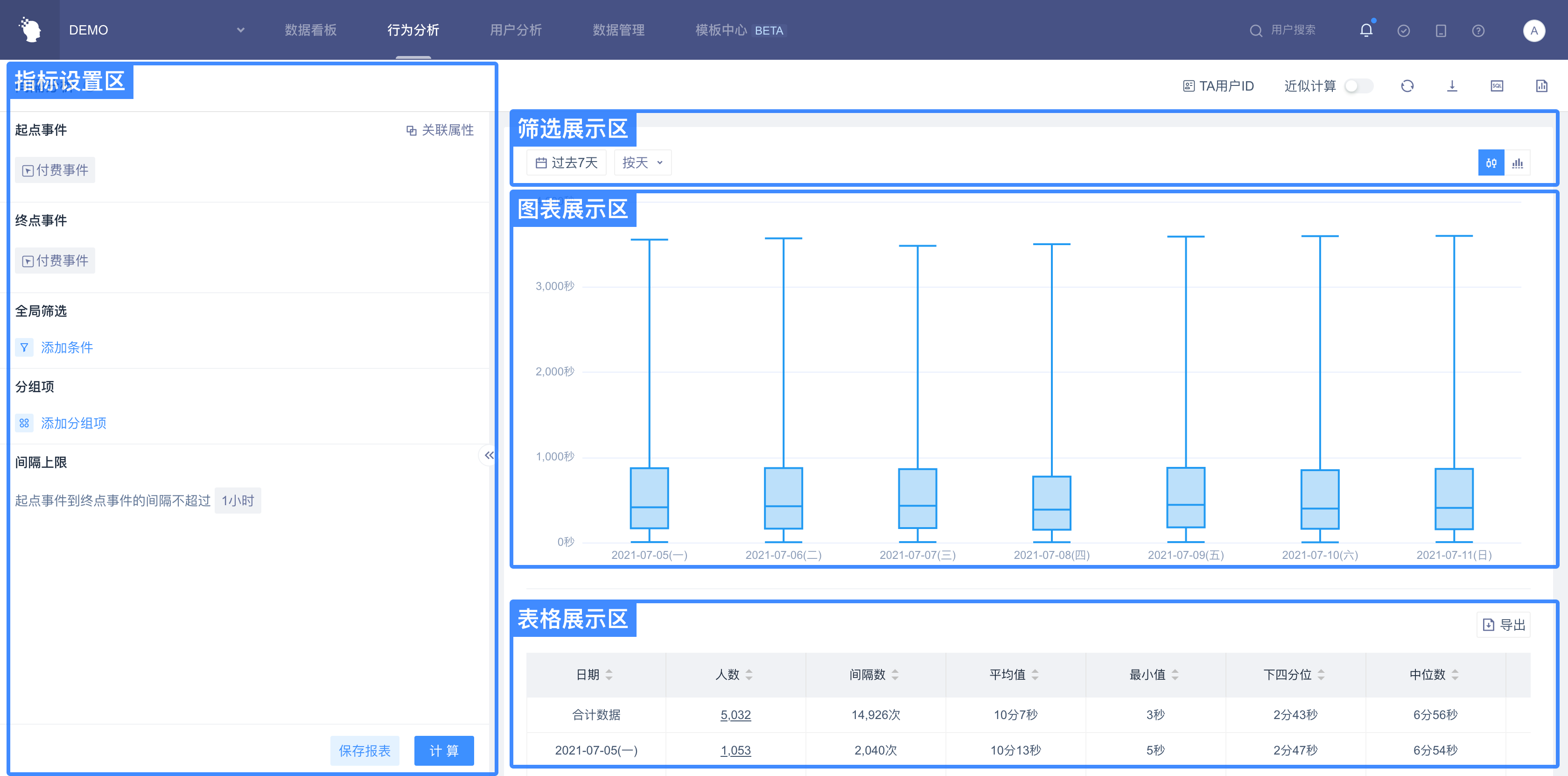
- The 'Indicator Settings Area' can set 'Start Event of Interval', 'End Event of Interval', 'Upper Interval', 'Interval Related Properties', 'Global Filter' and 'Group Items', etc.
- 'Display Filter Area' can set the calculation and display logic of icons and tables, and can adjust 'Analysis Time Period', 'Time Granularity', 'Group Settings', 'Chart Style', etc.
- In the 'Chart Display Area', you can choose the chart display form of the interval data. Currently, there are two chart display forms: 'Box-and-Whisker Plot' (ie. 'Box Plot') and 'Histogram'.
- The 'Table Display Area' will display the table data in the current chart display form, and the 'Box Plot' and 'Histogram' will have two different tables corresponding to each other.
# IV. Usage of Interval Analysis
# 4.1 Setting of Indicator Setting Area
# 4.1.1 Overview of the Indicator Setting Area
By default:
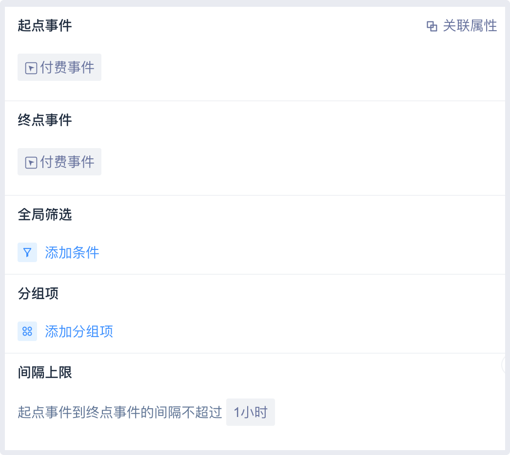
- 'Starting Event' and 'Ending Event' represent the starting and ending points of a time interval, which is equivalent to calculating the time difference between the starting event and the ending event; You can choose two different events or the same event, which will be different in algorithm.
- 'Global filtering' can filter both 'Starting Event' and 'Ending Event'. It can select 'Intersection of Event Attributes of Starting and Ending Event', 'User Attributes', 'User Groups' and 'User tags'.
- 'Grouping Items' can select 'Event Attributes for Starting Events', 'User Attributes', 'User Groups' and 'User tags'.
- The 'Upper Interval Limit' limits the calculated interval data and excludes data that exceeds the upper limit. By default, it is 1 hour. You can select the upper time limit by day, hour and minute in the drop-down box.
- The 'Interval Correlation Attribute' defines the attribute relationship between the starting and ending events of the interval.For example, if the attribute values of starting point and ending point are identical, the starting event and ending event with identical attribute values will be found in calculation.
# 4.1.2 Interval-related Attributes
In some analysis scenarios, it is necessary to stipulate the starting point and ending point of the calculation interval, and their attribute values need to meet certain conditions. For example, when calculating the two purchase intervals of the same commodity to analyze the purchase frequency of the commodity, it is necessary to set that the items purchased twice should be consistent. In the system, the commodity ID of the two behaviors of starting point and ending point can be set as the same, i.e., the set interval is the purchase interval of the same commodity.
Associated attributes need to select their respective event attributes from the starting event and the ending event respectively. The associated attributes of the two events can be different, but the attribute types need to be consistent.
'Associated Attributes of Starting Events' can select all types of event attributes in starting events, while 'Associated Attributes of Ending Events' can only select event attributes in ending events that are consistent with the type of 'Associated Attributes of Starting Events'. If you want to switch types, you need to switch from the 'Associated Attributes of the Starting Event'. After switching, the 'Associated Attributes of Ending Events' will also automatically switch to the corresponding type of event attributes.
The type of association attribute also determines the optional association relationship. All types can choose two association attributes to be equal. Numerical association attributes can also set the difference between attribute values, which can adapt to more analysis scenarios.
# 4.1.3 Upper Limit of Interval
The upper limit of the interval is equivalent to the set range of interval data, and the upper limit is equivalent to the maximum value. After the interval data calculation is completed, the data exceeding the upper limit will be excluded according to the interval upper limit.
The current upper limit configuration supports 'days (equivalent to 24 hours)', 'hours', 'minutes' three granularity, each granularity supports entering custom values.
In actual use, the upper limit of the interval may need to be adjusted many times and set in combination with the chart. A referential debugging process is to judge whether adjustment is needed by the distance between the upper quartile of the 'Box-and-Whisker Plot' and the maximum value, and then judge how much adjustment is needed by the interval near the maximum value in the 'histogram'.
# 4.2 Diagrams and Tables of Box-and-Whisker Plot
# 4.2.1 Display Filter Area of Box-and-Whisker Plot
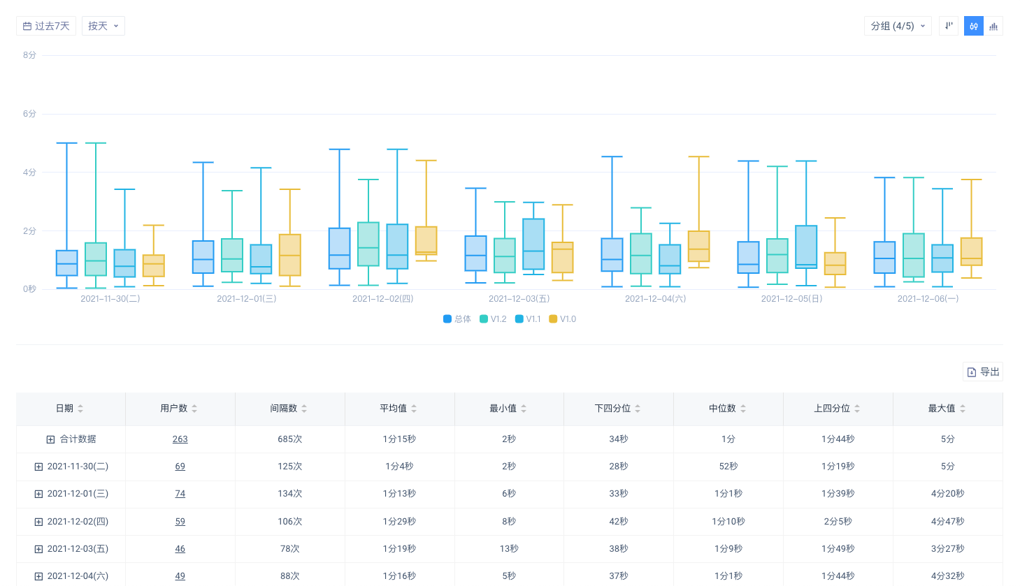
The box must diagram shows the distribution of interval data of different data series (dates and groups). The operation controls for the filter area are as follows:
- Analysis period
- Time granularity
- Grouping options
- Group sorting
- Chart switching
Analysis **P**eriod and **T**ime granularity
'Analysis Period' controls the time range of calculation. Starting events and ending events need to be affected by the time zone within this period of time.
'Time Granularity' controls the final time aggregation rules of the calculation results. You can choose 'by day', 'by hour', 'by week', 'by month' and 'total'. Among them, 'by week' can customize the start date of the week, and 'total' corresponds to the aggregation of results over a full period of time.
In particular, if 'Total' is selected for 'Time Granularity' of analysis and 'Group Items' are set, the upper limit of chart grouping options for 'Display Filter Area' will be released and 300 will be selected by default.
Group**ing** Options and Group Sorting
'Grouping Options' and 'Group Sorting' are displayed only when 'Group Items' are used in the calculation.
'Grouping Options' controls which data series the chart displays. You can select 'Total' and any group items. This operation is invalid for the table. The default selection includes the first 4 items including the 'Total' and the upper limit is also 4 items.
In particular, when the 'time granularity' is 'total', the upper limit of 'grouping options' will be released, defaulting to the first 300, with no upper limit.
'Group Sorting' can control the sorting rules in 'Grouping Options', which indirectly affects the contents displayed in the chart. The items that can be selected are 'Data Volume Upward', 'Data Volume Descending', 'Group Item Upward' and 'Group Item Descending'. The default is 'Data Volume Descending'.
# 4.2.2 Display Chart Area of Box-and-Whisker Plot
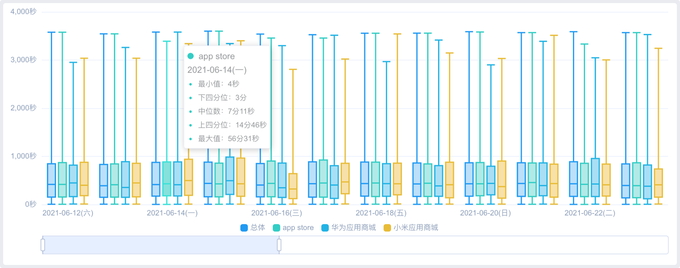
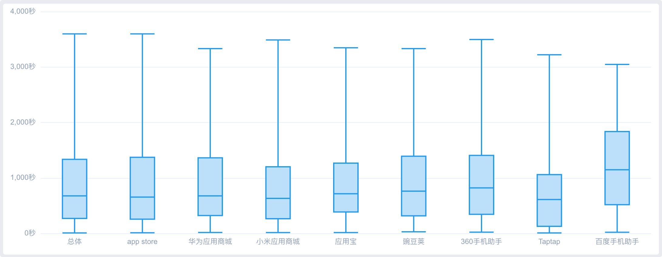
Boxes show aggregated data distributed over time intervals. A box must show 'maximum', 'upper quartile', 'median', 'lower quartile' and 'minimum'. The hovering float will show the same thing. When 'time granularity' is not 'total', the time dimension acts as an inter-group dimension. Data are clustered by time, and the horizontal coordinate also shows the time dimension. The grouped items are intra-group dimensions.
In particular, when the 'time granularity' is 'total' and 'group items' are set, then the horizontal coordinates of the chart will be replaced by grouped items from dates as shown in the following diagram:
# 4.2.3 Display Table Area of Box-and-Whisker Plot
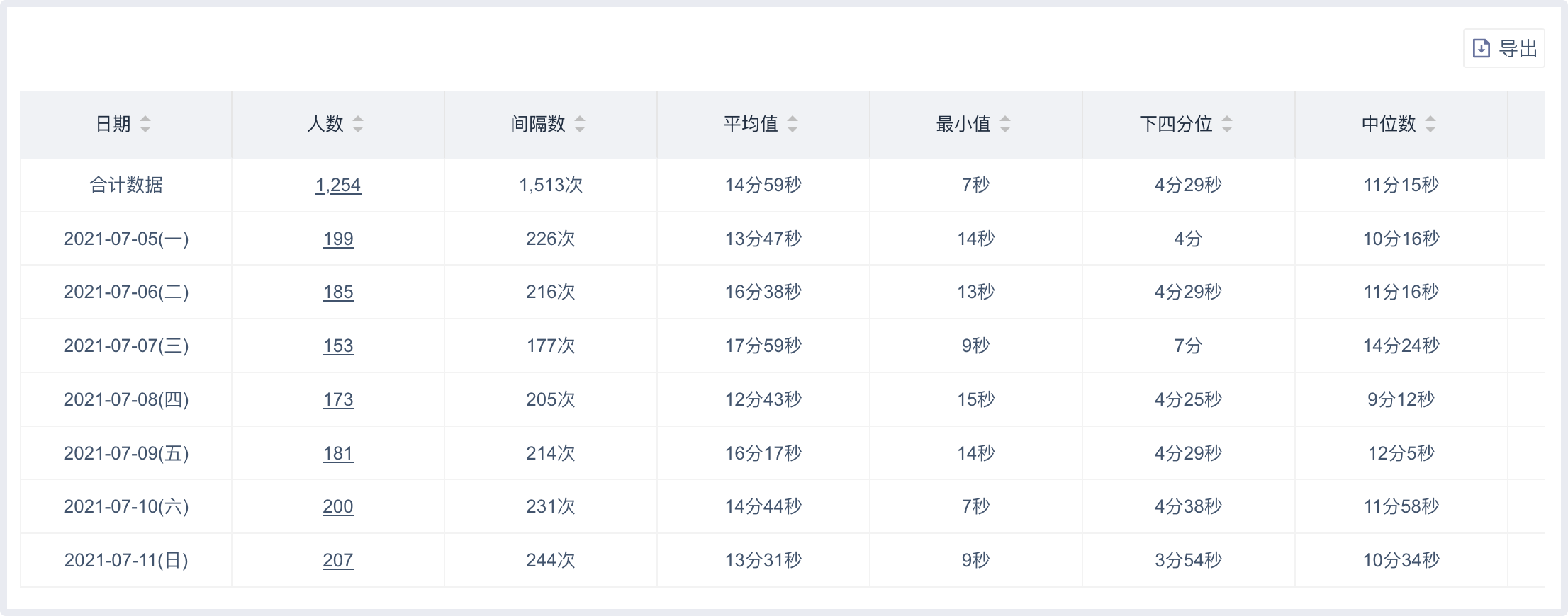
As shown in the table above, the data shown in the Box-and-Whisker Plot are 'Number of people', 'Number of intervals', 'Average value', 'Maximum value', 'Upper quartile', 'Median', 'Lower quartile' and 'Minimum value'. The number of people can be clicked into the 'User List'. In addition, the full-time aggregate data will be displayed.
If you need to export the table data, you can click the 'Export' button at the top right of the table to export the table data in a table format (the table data only shows the first 1000 and the export only exports the first 1000, so you can download more data using Data Download in the upper right corner of the page).
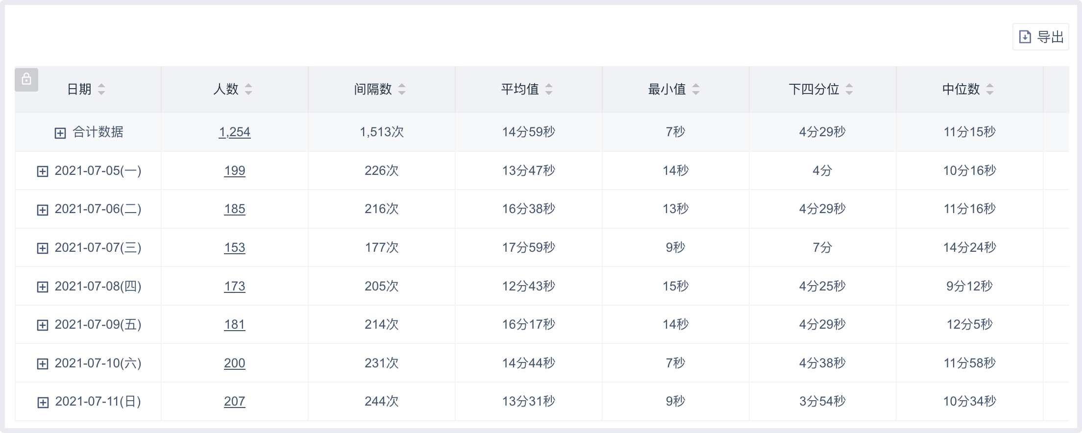
If 'Group Item' is set and 'Time Granularity' is not 'total', the grouped data needs to be displayed through the floating window by clicking '+' sign in front of the time column.
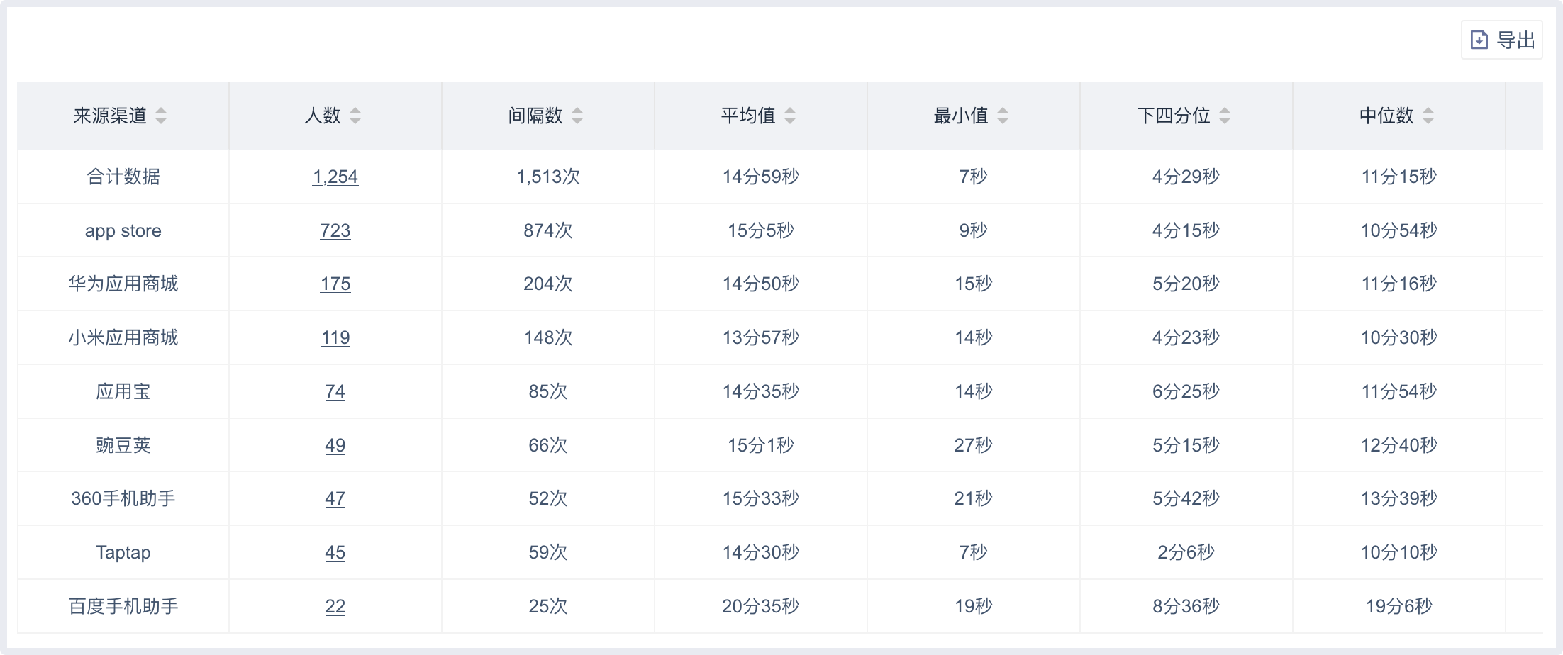
If 'Group Items' is set and 'Time Granularity' is 'Total', the time column will be replaced by the group column, and the grouped data will be displayed directly in the table.
# 4.3 Histogram Charts and Tables
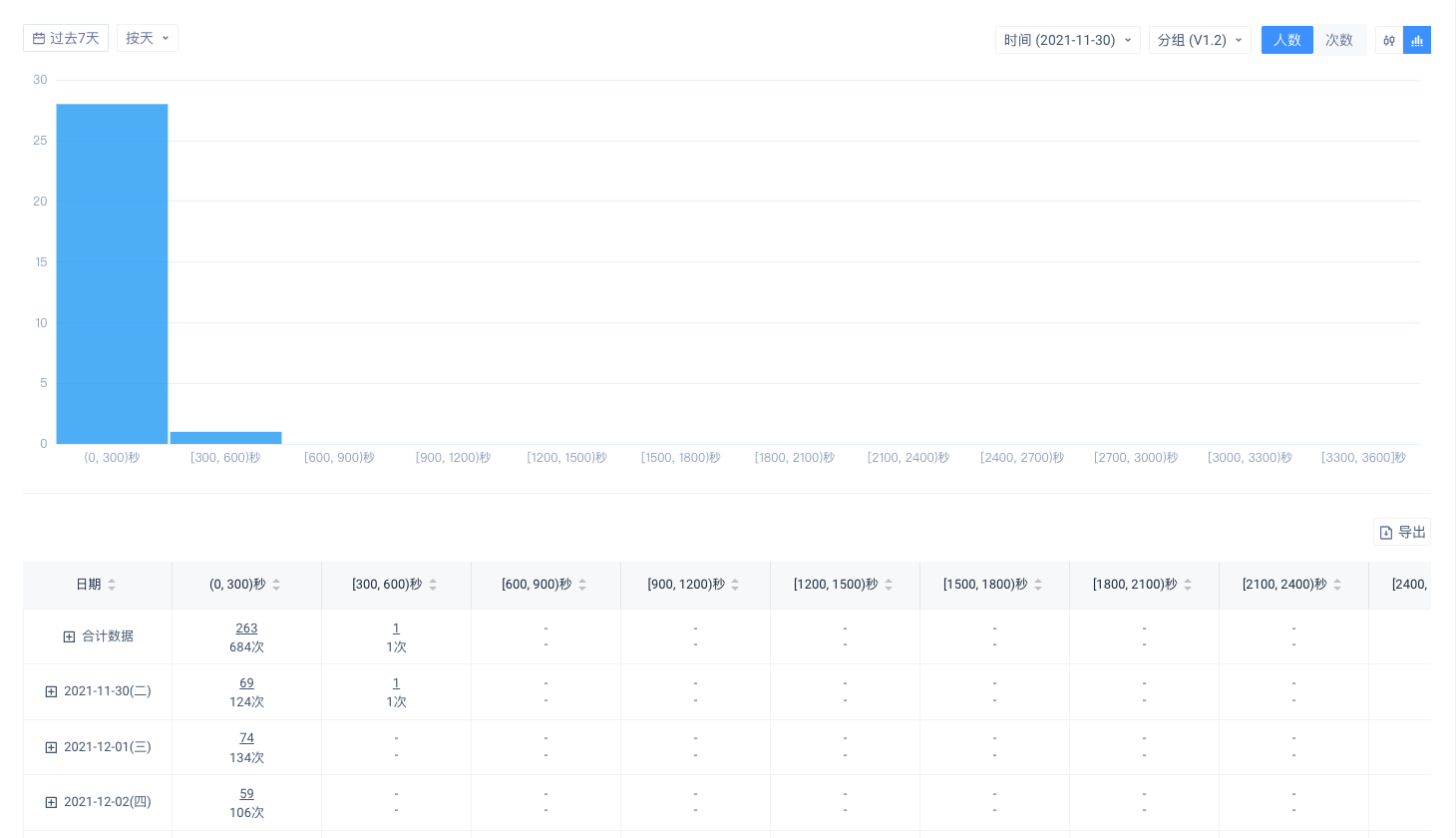
# 4.3.1 Histogram Display Filter Area
The histogram shows the distribution of interval data for a data series (date and group). The operation controls showing the filter area are as follows:
- Analysis period
- Time granularity
- Grouping options
- Time options
- Number of people Switching
- Chart switching
Analysis **P**eriod and **T**ime **G**ranularity
'Analysis Period' controls the time range of calculation. Starting events and ending events need to be affected by the time zone within this period of time.
'Time Granularity' controls the final time aggregation rules of the calculation results. You can choose 'by day', 'by hour', 'by week', 'by month' and 'total'. Among them, 'by week' can customize the starting date of the week, and 'total' corresponds to the aggregation of results over a full period of time.
Group Options and Time Options
'Group Options' will only be displayed when 'Group Items' are used in the calculation. 'Time Options' will only be displayed when 'Time Granularity' is not 'Total'.
Since the histogram only displays one data series, the 'Group Options' and 'Time Options' can only be selected by radio. The two controls specify which data series to display.
'Grouping Options' controls the grouping items of the data series. You can select 'Total' and any group items. It is invalid for the table. By default, "Total" is selected.
The "Time Option" controls the time of the data series. You can select "Total" and all the time of the analysis period. This operation is invalid for the table. 'Total' is selected by default.
Number of **P**eople Switching
The 'Number of People Switch' control can switch whether the data in the histogram shows the number of people or the number of intervals.
# 4.3.2 Display Chart Area of Histogram
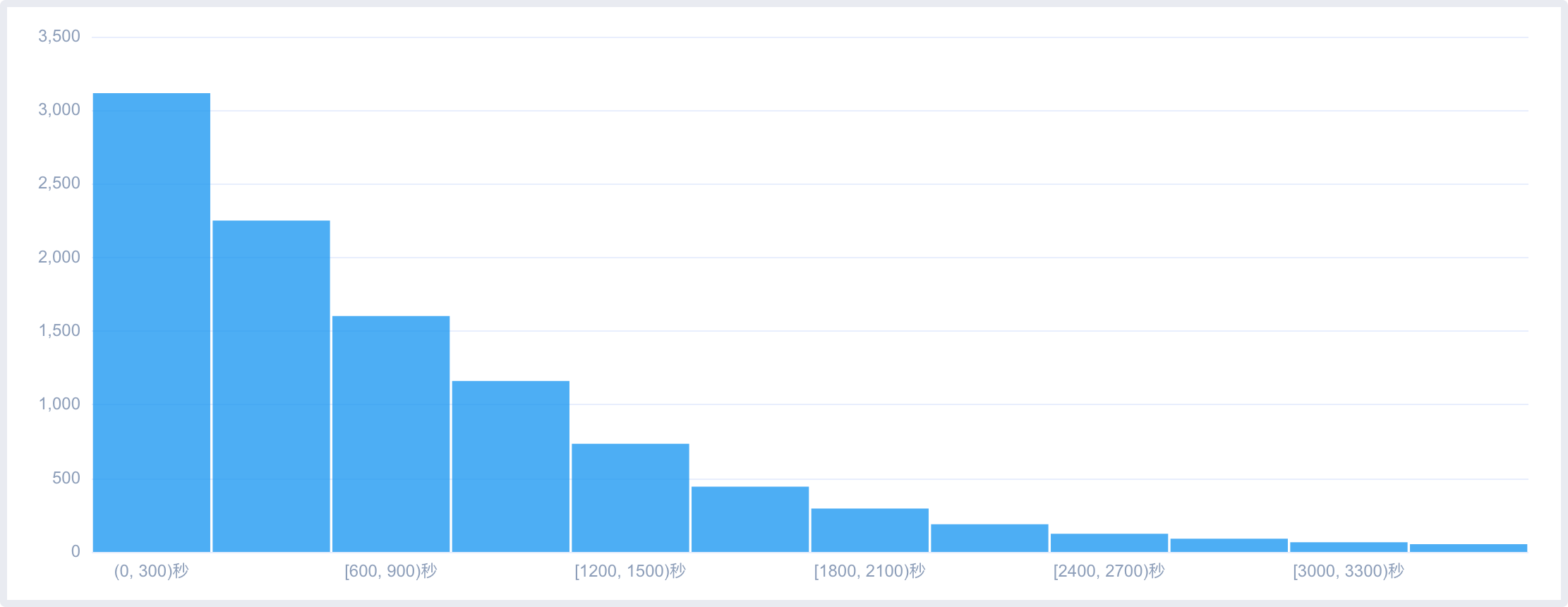
The histogram shows the interval distribution of a data series, and it is a histogram of frequency distribution with equal group spacing. The data range is 0 to the upper interval limit. The number of groups is currently limited to 12 groups. Whether the group has data or not, it will be displayed in the figure.
Through the 'Number of People Switching' control, you can switch whether the frequency displayed by the histogram is the number of people or the number of intervals.
# 4.3.3 Display Table Area of Histogram
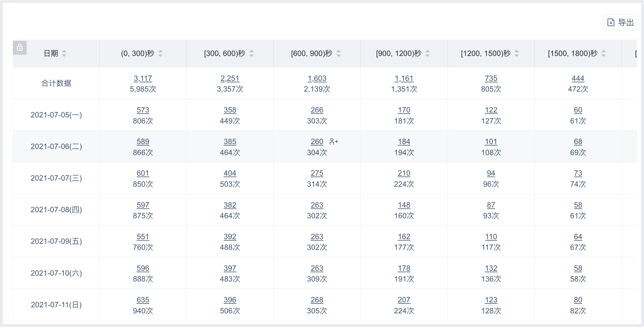
Histogram shows the interval distribution of a series of data, and it is a histogram of equal frequency distribution with group spacing. The data range is 0 to the upper limit of interval, and the number of groups is limited to 12 groups. Whether the group has data or not, it will be shown in the diagram.
If you need to export the table data, you can click the 'Export' button at the top right of the table to export the table data in a table format (the table data only shows the first 1000 and the export only exports the first 1000, so you can download more data using Data Download in the upper right corner of the page).
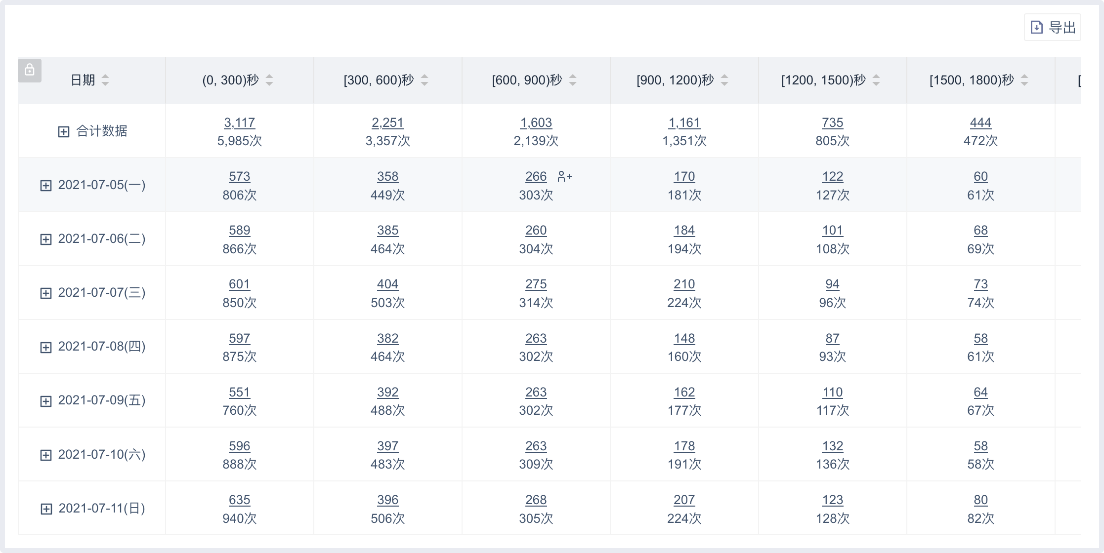
If 'Group Item' is set and 'Time Granularity' is not 'Total', the grouped data needs to be displayed through the floating window by clicking "+"sign in front of the time column.
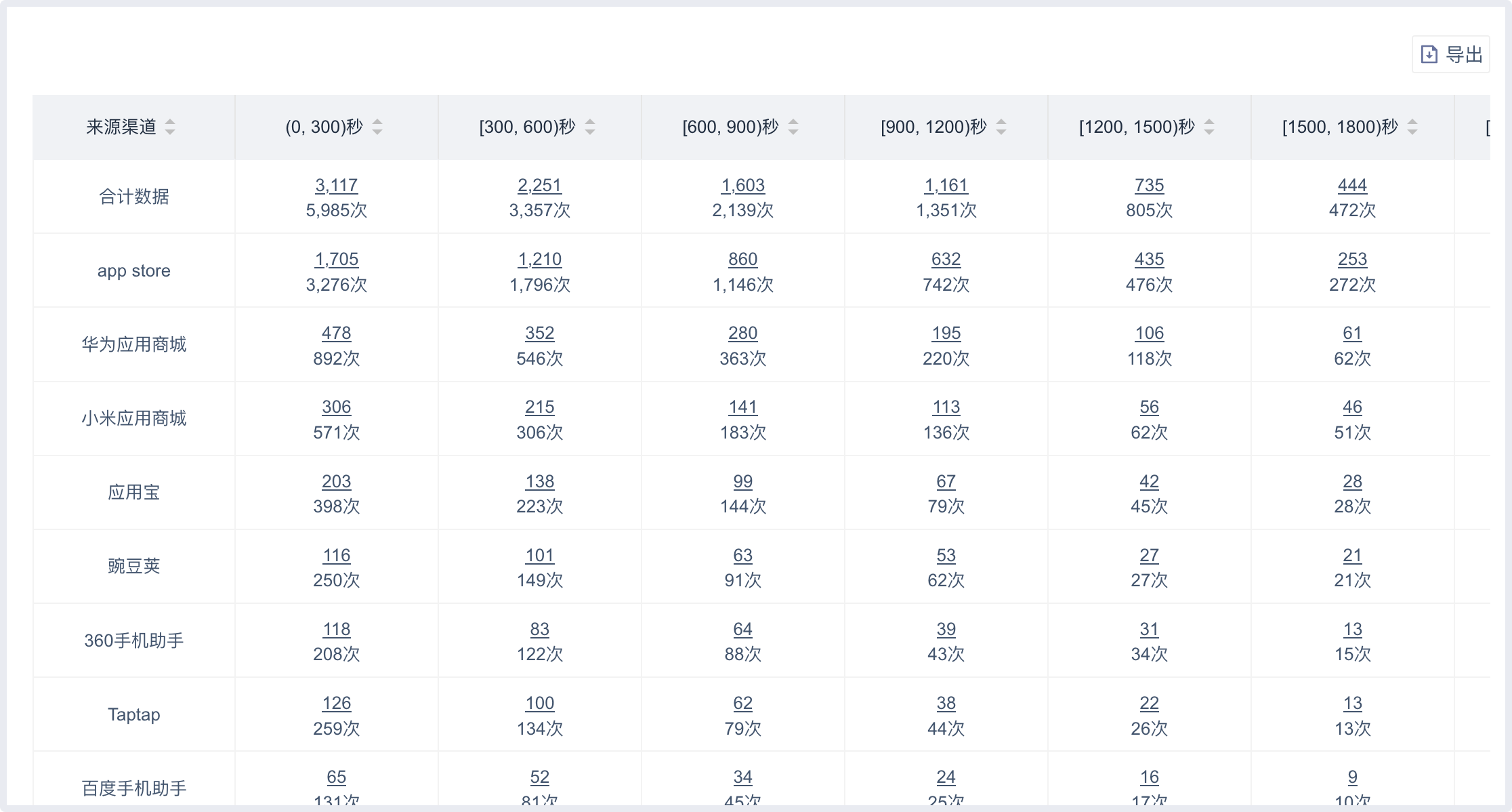
If 'Group Items' is set and 'Time Granularity' is 'Total', the time column will be replaced by the group column, and the grouped data will be displayed directly in the table.
# V. Computational Logic of Interval Analysis
The logic of interval analysis can be divided into two categories, one is the conventional interval calculation, which is suitable for scenarios with different starting and ending points. The other is more special and applies to scenarios where the starting and ending events are identical, i.e. the same event. This section will introduce these two kinds of computational logic.
# 5.1 Different Intervals between Starting and Ending events
# 5.1.1 Shortest Interval Principle
Assuming that the starting event of the interval is A and the ending event is B, the user's behavior sequence is as follows:
| Behavioral sequence | 1 | 2 | 3 | 4 | 5 | 6 |
|---|---|---|---|---|---|---|
| Behavioral events | A | A | B | A | B | B |
When calculating the interval, we will maintain the 'shortest interval principle', which can also be called the 'proximity principle'. When two consecutive starting point events occur, the former starting point event will be excluded and the interval will be calculated from the latter starting point event. However, if two consecutive ending events occur after a starting point event, the interval calculation will only be carried out with the previous ending event. Based on this principle, it can be ensured that the interval is the shortest.
The above sequence of behaviors produces the following two intervals.
| Behavioral sequence | 2 | 3 |
|---|---|---|
| Behavioral events | A | B |
| Behavioral sequence | 4 | 5 |
|---|---|---|
| Behavioral events | A | B |
TIP
There are two reasons for adopting the 'shortest interval principle'. One is to make the interval more reflective of the meaning of transformation, and the principle of proximity is most commonly used in transformation, i.e. the most recent behavior has the greatest impact on subsequent behavior. The second is to reduce the impact of interval data when data is missing. If the sequence of behaviors is a standard A-B alternating behavior stream, the proximity principle can minimize the problem of data anomalies caused by one of the behaviors being lost.
# 5.1.2 Time Deduplicate Principle
If there are multiple starting events that have exactly the same trigger time, they are treated as the same behavior and only the interval is calculated once.
If a starting event coincides exactly with the trigger time of the ending event, the ending event will be skipped, and the ending event will continue to be searched backward and the interval will continue counting.
Adopting the 'time deduplicate principle' actually means that the behaviors at both ends of the interval cannot be triggered at the same time, otherwise the interval cannot be calculated and the meaning of transformation cannot be reflected. If the time is the same due to the time accuracy issue, millisecond recording behavior is recommended.
# 5.1.3 Computational Logic for Starting and Ending events at Different Times
Assuming that the starting event of the interval is A and the ending event is B, to ensure that no multiple behaviors occur at the same time, the user's behavior sequence is as follows:
| Behavioral sequence | 1 | 2 | 3 | 4 | 5 | 6 | 7 | 8 | 9 | 10 |
|---|---|---|---|---|---|---|---|---|---|---|
| Behavioral events | A | B | A | A | B | C | B | A | C | B |
Each starting event A will look for the ending event B backwards. During this period, following the 'shortest interval principle' and 'time deduplicate principle', the 4 pairs of A-B behavior produce 3 intervals, namely:
| Behavioral sequence | 1 | 2 |
|---|---|---|
| Behavioral events | A | B |
| Behavioral sequence | 4 | 5 |
|---|---|---|
| Behavioral events | A | B |
| Behavioral sequence | 8 | 10 |
|---|---|---|
| Behavioral events | A | B |
The A events of sequence 3 and the B events of sequence 7 are excluded due to the 'shortest interval principle'.
# 5.2 The Interval when Starting and Ending Events are the Same Event
The starting event and the ending event need to be the same event, and the filter conditions need to be consistent, but the filter order can be different.
However, it should be noted that logically identical events may not necessarily be considered the same event. For example, starting events are filtered by events and ending events are selected by a logically identical virtual event, and then different events are considered. The former algorithm is adopted.
Assuming that the starting event and the ending event of the interval are both A, to ensure that no multiple behaviors occur at the same time, the user's behavior sequence is as follows:
| Behavioral sequence | 1 | 2 | 3 | 4 | 5 | 6 | 7 | 8 | 9 | 10 |
|---|---|---|---|---|---|---|---|---|---|---|
| Behavioral events | A | B | A | A | B | C | B | A | C | B |
Each event A will look for another event A backwards, and an event A can be used as the starting point of an interval or the end point of an interval. Following the 'time deduplicate principle', the 4 A events produce 3 intervals, respectively:
| Behavioral sequence | 1 | 3 |
|---|---|---|
| Behavioral events | A | A |
| Behavioral sequence | 3 | 4 |
|---|---|---|
| Behavioral events | A | A |
| Behavioral sequence | 4 | 8 |
|---|---|---|
| Behavioral events | A | A |
Under the 'time deduplicate principle', it can be assumed that there will be an A-1 interval when there are certain events A.
# 5.3 Introduction of Associated attributes and Grouping
Introduction of associated attributes and grouping will not change the core logic of the above calculation. The two functions are logically similar, but the processing is different.
The introduction of associated attributes will be carried out before the interval calculation. First, all original data sources will be grouped according to associated attributes, and then the interval calculation will be carried out within each group. The packet entry is the interval data packet after the interval calculation is completed. Because grouping takes place at different times and does not interfere with each other, association attributes and grouping can also be used at the same time.
# 5.4 Upper Interval Limit
The upper limit of the interval is carried out after the calculation interval is completed. The interval data exceeding the upper limit will be eliminated, grouping and aggregation will be carried out only after the data is eliminated.
# VI. Best Applications
# 6.1 New User Payment Conversion Interval
Interval analysis can be used as a supplement to the funnel for important conversions, such as the first payment after new users register. The conversion duration can be carefully analyzed through interval analysis to understand the conversion duration, which can not only evaluate the effect of ice-breaking payment, but also use this indicator as a key focus indicator to evaluate the conversion of new users.
# 6.2 Time Length of Behaviors
If an actual behavior records the beginning and end of the behavior, such as entering a product page, exiting a product page, or more common, opening and closing an application. Actual behavior like this can be calculated over time using interval analysis, just by setting the starting and ending of the behavior as the starting and ending events of the interval.
# 6.3 Dwell Time
In your game or application, users may be in a state of hierarchy/ladder for a long time, such as a hierarchical membership system. A user may maintain a low level for a period of time before rising to a high level, such as 'Silver Member' upgraded to 'Gold Member'. Such a hierarchy/ladder system is extremely common, including the above-mentioned membership level, beginner's guide steps, play level progress, course completion progress, etc., are adopted by various products. We can call the time interval from one stage to the next in this system the dwell time, i.e. how long a user stays at a certain stage. Such dwell analysis can be easily constructed by interval analysis and reasonable use of association attributes and grouping.
